
Geofencing at Scale: QuadTrees, Geohashes, and Real-Time Location Tracking
The Hidden Complexity Behind “You’ve Arrived”
You’ve ordered food delivery. The app shows your driver’s location updating every second as a little car icon creeps closer. When they’re within 100 meters, you get a notification: “Your driver is nearby!” Behind this seemingly simple feature lies one of distributed systems’ most demanding challenges: tracking millions of moving objects and instantly knowing which ones entered or exited invisible boundaries. When Uber processes 100+ million location updates daily or DoorDash monitors hundreds of thousands of active deliveries simultaneously, the naive approach of checking every location against every boundary creates an O(n²) nightmare that would melt servers.
How Spatial Indexing Tames Coordinate Chaos
The fundamental problem: given a coordinate (latitude, longitude), which polygonal regions contain this point? Checking every geofence sequentially becomes prohibitively expensive at scale. This is where spatial indexing transforms impossibility into practicality.
Geohashes reduce two-dimensional coordinates to a single string through clever bit-interleaving. The algorithm alternates between longitude and latitude bits, creating a Z-order curve that preserves spatial locality. A geohash like “9q5” represents a specific region, and nearby locations share longer common prefixes. For example, “9q5csy” and “9q5cst” are neighbors, while “9q5csy” and “dqcjq” are far apart. This prefix property enables lightning-fast range queries: finding all points within a region becomes a simple string prefix match rather than complex geometric calculations.
The encoding precision matters critically. Each additional character in the geohash divides the area into 32 smaller cells (5 bits per character). A 6-character geohash represents roughly 1.2km × 0.6km, while 8 characters narrows to 38m × 19m. Systems must balance precision against storage and query performance—too precise and you’re checking too many cells, too coarse and you get false positives requiring expensive geometric verification.
QuadTrees take a different approach through recursive spatial subdivision. Start with the entire map as a single node. When that node contains too many objects (typically 4-16), split it into four equal quadrants: NW, NE, SW, SE. Each quadrant recursively subdivides as needed. This creates a hierarchical structure where sparse areas remain coarse-grained while dense urban centers subdivide deeply.
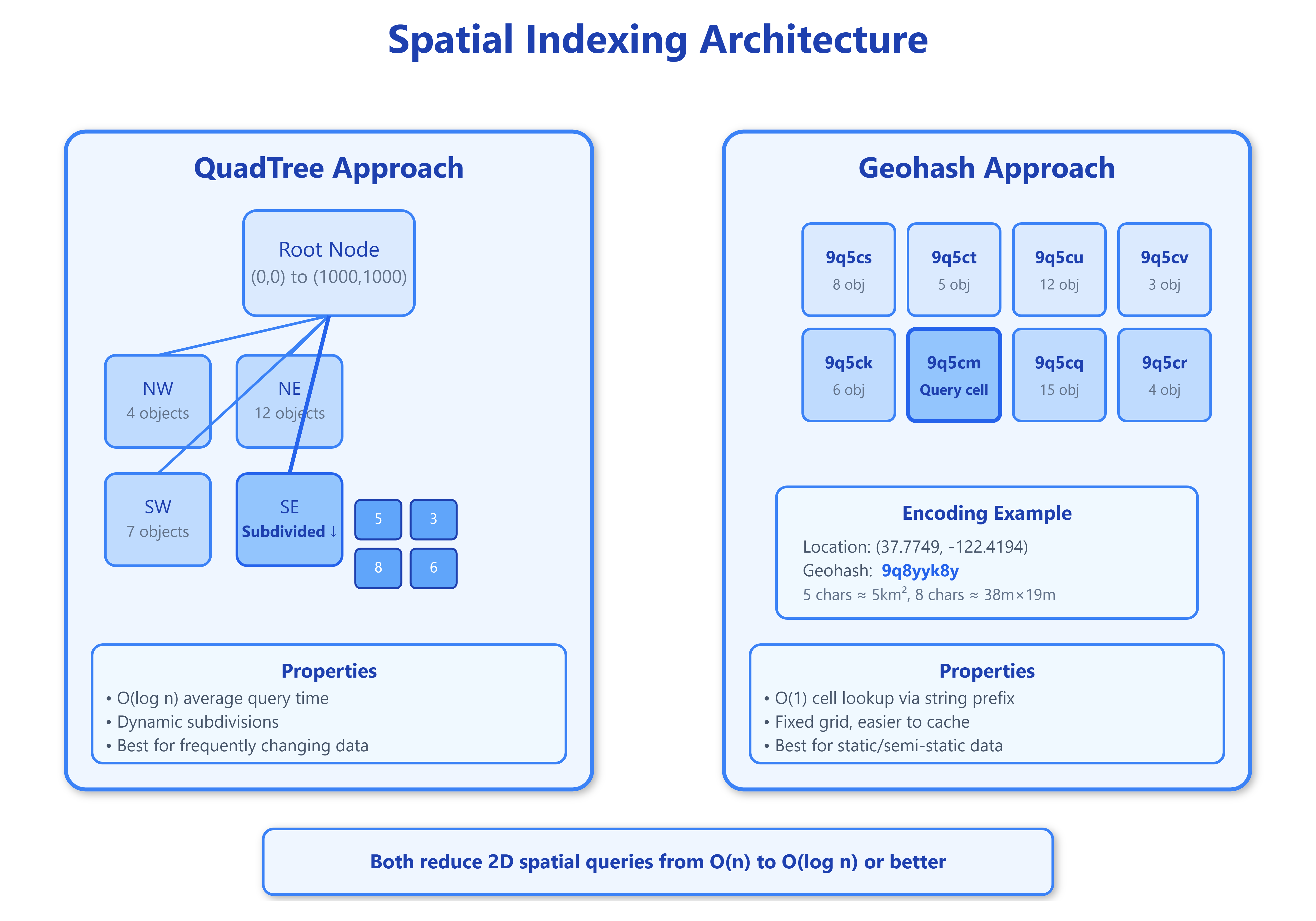
The elegance emerges during queries. To find objects near a point, traverse the tree from root to leaf, only exploring relevant quadrants. The average case is O(log n), but the worst case—all objects clustered in one quadrant—degrades to O(n). Real systems hybrid-proof this by switching to geohashes when a quadrant becomes pathologically deep.
S2 Geometry (Google’s approach) extends these concepts with spherical geometry, avoiding distortions from projecting a sphere onto a plane. S2 cells form a hierarchical grid on the sphere itself, maintaining consistent area regardless of latitude. This matters at global scale—geohashes near poles have vastly different areas than equatorial ones with identical precision.
Critical Insights: What Breaks at Scale
Common Knowledge:
Both QuadTrees and Geohashes reduce two-dimensional search to manageable complexity. They’re not competing technologies but complementary—QuadTrees for dynamic, rapidly changing object sets; Geohashes for indexing massive static datasets in databases.
Rare Knowledge:
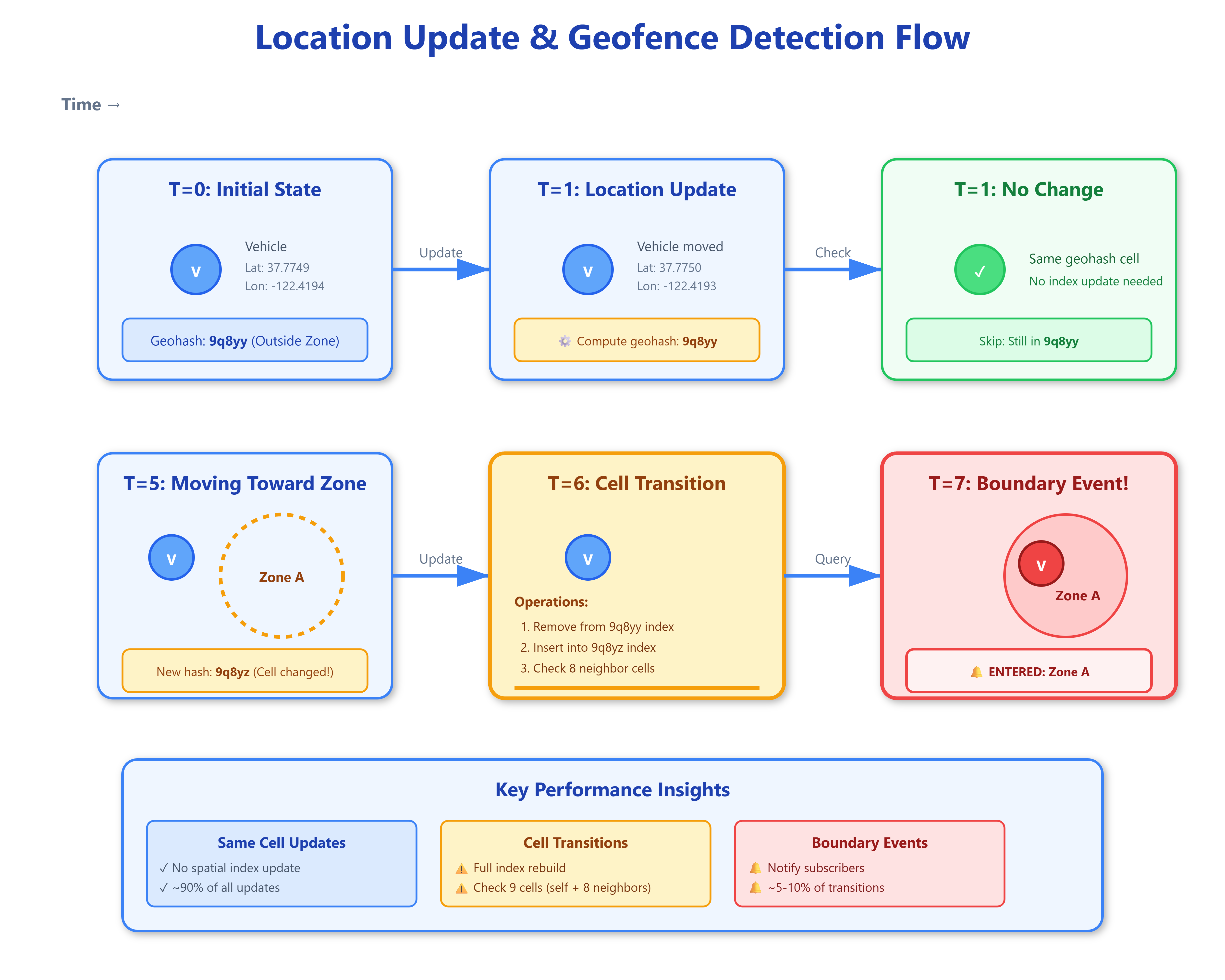
The real killer isn’t query performance but update storms. When a driver moves from one geohash cell to another, you’re not just updating coordinates—you’re removing from one spatial index, inserting into another, potentially notifying all subscribers to both cells, and invalidating various caches. At 100 million updates daily, even 1ms per update means 27+ hours of CPU time. Solutions involve delta compression (only send updates when movement exceeds a threshold), predictive indexing (pre-compute likely next cells), and batched updates (accumulate changes, flush periodically).
Advanced Insights:
Geofence boundaries rarely align with geohash cell edges. A point might be in cell “9q5csy” but the geofence polygon straddles multiple cells. This creates the “boundary problem”: you must check adjacent cells during queries, multiplying I/O operations. Clever systems maintain a “buffer zone”—geofences are indexed in all cells they touch plus a margin. This trades storage (redundant indexing) for query simplicity (no adjacency checks).
Strategic Impact:
Location update latency compounds across the stack. GPS sampling delay (1-5 seconds), network transmission (100-500ms), geohash computation (microseconds), database write (10-50ms), pub/sub propagation (50-200ms), and client rendering (16ms for 60fps) sum to multi-second end-to-end latency. Systems can’t eliminate these delays but must design around them—showing predicted positions, implementing client-side interpolation, and accepting eventual consistency.
Implementation Nuances:
Most production systems use a three-tier approach: PostgreSQL with PostGIS for authoritative geofence storage, Redis with geospatial commands for hot-path queries, and in-memory QuadTrees in application servers for sub-millisecond lookups. Redis GEOADD and GEORADIUS provide decent performance (thousands of queries/second per node) but don’t handle complex polygons. Complex shapes get decomposed into multiple simpler geohashes or stored in PostGIS for occasional verification.
Real-World Examples
Uber processes 100+ million location updates daily across their driver network. They use a hybrid system: S2 cells for coarse global partitioning, geohashes for city-level indexing, and in-memory QuadTrees for active trip tracking. Their “supply positioning” system pre-computes probable driver locations 5 minutes ahead, indexing future positions to reduce cache misses during demand spikes.
DoorDash handles “arrival detection” for hundreds of thousands of simultaneous deliveries. They discovered that naive geofence checking caused 40% of their location update CPU load. Solution: geohash-based prefiltering reduced candidate geofences from thousands to typically 3-5, then exact polygon intersection only on candidates. Update latency dropped from 150ms to 12ms p99.
Lyft deals with “zone pricing” where different map regions have different surge multipliers. Riders moving between zones must see instant price updates. They maintain a regional geohash index replicated across multiple Redis clusters. Each location update triggers a Bloom filter check (eliminating 95% of zone-boundary-crossing checks) before expensive polygon verification.
Architectural Considerations
Spatial indexing isn’t isolated—it’s deeply coupled with your entire location infrastructure. Monitoring requires tracking not just query latencies but spatial distribution of updates (hot spots can overwhelm single nodes), index depth distribution (unbalanced QuadTrees signal problems), and geohash collision rates (too coarse means wasted computation).
Cost implications are non-trivial. PostGIS with proper spatial indexes requires 3-5× more storage than raw coordinates. Redis geospatial adds 50-100 bytes per entry versus simple key-value. At billions of tracked objects, this compounds to substantial memory costs. Many systems archive cold locations (unmoving objects after N hours) to cheaper blob storage, rehydrating only when they activate.
Use QuadTrees when you need sub-millisecond in-memory lookups with frequently changing object sets (active vehicles, nearby player matching). Use Geohashes when you’re querying persistent datasets at moderate frequency with database backing (restaurant locations, service areas). Use S2 for truly global applications spanning multiple continents where projection distortions matter. For most city-scale applications, Geohashes provide the best balance of simplicity and performance.
Practical Takeaway
GitHub Link:
https://github.com/sysdr/sdir/tree/main/Geofencing_at_Scale/geofence-demoStart by profiling your specific access patterns—are you doing more location updates or geofence queries?
Different ratios demand different optimizations. For initial implementations, Redis geospatial commands provide excellent bang-for-buck, handling thousands of operations per second on a single node. Graduate to dedicated spatial databases only when you’ve proven Redis can’t scale to your load.
Run bash setup.sh to see a complete geofencing system in action. The demo implements both QuadTree and Geohash approaches side-by-side, simulating 1,000 moving vehicles and multiple geofenced zones. Watch how each algorithm handles boundary crossings, observe the different query patterns, and compare performance metrics in real-time. The dashboard visualizes both spatial indexing structures, showing how they partition space differently and highlighting trade-offs. Extend the demo by adjusting geohash precision, modifying QuadTree node capacity, or adding complex polygon geofences to see how each approach scales.
The key insight:
Spatial indexing isn’t about choosing “the best” algorithm but understanding which trade-offs align with your specific constraints. Master these fundamentals and you’ll build location systems that scale from hundreds to millions of tracked objects without breaking a sweat.